Optimizers we build
Humans do not optimize. They do not have computers in their brains that help with decision making. In fact, it's not clear how we do all the amazing stuff we do everyday. However, we do know given time and stakes, humans build systems that actually optimize. Delegated optimization is most of what engineering is.
Economics went the other way. For a century it modeled human choice as if the human were the optimizer, then built an entire estimation apparatus on top of that assumption. I have spent a lot of my life inside that apparatus. This post is about why I stopped believing the usual story I tell about it, and what changed my mind back.
The post I could not write
The arc was the following: modern machine learning is pattern recognition. It will fail when we move to environments it has never observed, because it has no model of the mechanism generating the data, only the data. And then structural econometrics provides the solution: structural models estimate primitives that are stable across regimes and therefore robust to the Lucas critique.
Here is the problem. We cannot say that humans optimize anything in particular. So every equilibrium model rests on an assumption we have no way to confirm. Worse, we can almost never run the experiment that would test it, the intervention that pushes behavior to a genuinely new equilibrium and checks whether our estimated primitives predicted the move. Absent that, a structural model is an internally consistent story we cannot falsify. I was going to sell robustness to a critique while quietly relying on an assumption at least as fragile as the one the critique attacks.
What actually changed
Now decisions are increasingly made by synthetic agents that do in fact optimize. A reinforcement learning agent solving a Markov decision process is, unlike a person, actually computing a policy that maximizes a discounted objective.
The optimizing-agent assumption was always the weak joint in structural economics. When a firm delegates a decision to an RL agent, that assumption stops being an idealization of a human and becomes a literal description of the machine. The human encodes what she wants into a reward and delegates the optimization to something that will actually execute it.
Structural econometrics does not become valid because humans became optimizers. It becomes valid because the decision-makers did. As delegation spreads, the share of economically consequential behavior that is genuinely optimizing grows, and a toolkit built on that assumption finally finds the domain where the assumption is true rather than hoped for.
An old idea, made literal
In the early 1980s Margaret Bray asked whether rational expectations, the assumption that agents know the equilibrium mapping of the economy they inhabit, could be justified rather than assumed. Her answer: suppose agents do not know the mapping but estimate it, running least squares on the data the economy itself generates and acting on the forecast. The summary is that rational expectations is what you get if the agents are econometricians.
We now inhabit this world even more directly. The pricing agent is not metaphorically running an estimation loop, it is actually running one. Bray's econometrician-agent, imagined to rationalize equilibrium, is now deployed in production.
A concrete setting
Imagine I run a marketplace. Third parties sell on it and set their own prices, using whatever technology they like. As the owner, I want to know how participants will respond if I change the rules. This is the classic structural question. The difference is that here it has a real chance of capturing the true nature of the agents, because the agents are, by construction, the kind of thing my methods assume.
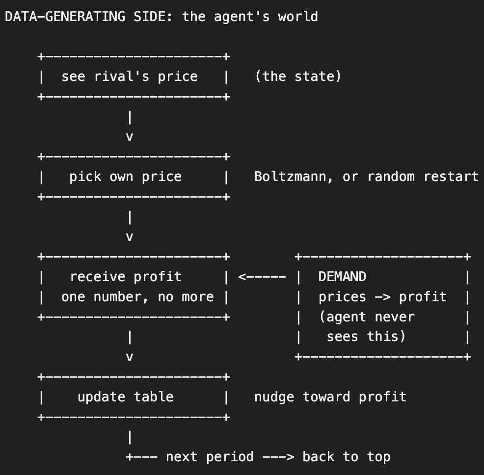
Take two firms that delegate pricing to agents. Each firm inputs its marginal cost and hands the agent a reward equal to profit. The agent sets a price, the market returns a quantity, profit is margin times quantity. Crucially, the agent does not know the demand function. It only ever sees the scalar that comes back. Prices are set in alternating moves, which captures the fact that firms' decision epochs need not line up. The agents learn by entropy-regularized Q-learning, a pretty popular choice.
The reward channel is the whole point. A single number enters the update. Demand sits outside the loop, shaping that number, never seen by the agent. The firm's private primitive, marginal cost, lives one level further out still, inside the reward the human specified.
A Surprising Equivalence
Here is the fact that makes the setting more than an analogy. The choice rule that entropy-regularized Q-learning converges to is the same object that structural econometrics has been inverting for forty years.
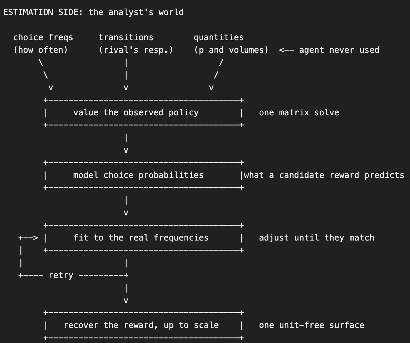
Soft Q-learning replaces the hard maximum in the Bellman update with a log-sum-exp, and its stationary policy is a Boltzmann distribution over actions. Write that policy down and it is exactly the choice probability of a dynamic discrete choice model with additive type-one extreme value shocks.
So the estimator built to recover human preferences is, formally, the inverse of the algorithm the firms deployed.
On simulated play from two alternating-move soft-Q agents, the inversion recovers what the agents were optimizing. But it recovers less than it first appears, and understanding exactly how much less is the whole story.
What behavior can and cannot hand you
Here is the catch, and it is the oldest result in discrete choice wearing new clothes. The agent chooses by weighing each price's payoff against a random exploration shock. Invert the behavior and you recover the payoff, but only divided by the scale of that shock. Double the payoffs and double the noise and nothing an observer sees changes, so that scale is never identified; it is normalized by hand. In the classical setup the scale is an abstract nuisance. Here it has a name, the exploration temperature, the knob that sets how sharply the agent chases the best price. It is a real primitive, it governs the choices, and it is exactly the thing the data will not pin.
This is cleaner than the usual structural story, not messier. The recovery needs no functional form: it returns a payoff surface, a number for every price in every state, and never asks what that payoff is made of. I do not assume it is profit, or price minus a constant cost times quantity, or anything about its shape. And no amount of extra data buys back the scale. My platform even clears the trades, so it sees every price and quantity, yet the scale still sits on everything. (The full accounting, a per-state level and the discount factor alongside the scale, is in the appendix; only the scale matters for what follows.)
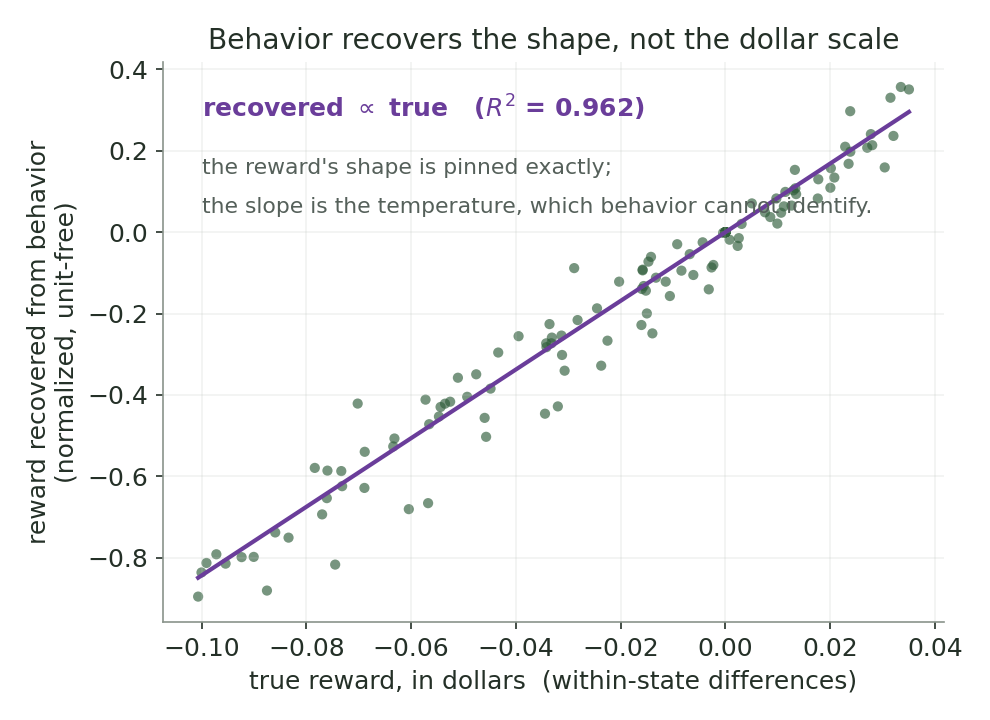
The picture shows how this plays out. The choices allow me to invert back the rewards in a scale free manner. The real reward function is in dollars and we cannot get at that from the choices. The inversion is working out, for each state configuration we are closely mapping back to the true reward, i.e. each point is close to solid line. But the line does not have a slope of 1, the recovered reward is a transformation of the true one. But we do not know what the parameter is that generated that transformation. This is the free parameter of the q learning bot.
The move that rescues this is to stop demanding a dollar figure and ask a different question. For any given rule change I might want to test, is the answer a pure number that the normalized reward already contains, or does it require a dollar scale I do not have? That is a property of the question, not of the estimate, and it splits the marketplace owner's levers along exactly the line the picture drew. Interventions that only re-scale or reorder the reward are answerable. Interventions that add or subtract dollars are not, at least not without pinning the missing scale.
Let us focus on the latter: charge a flat fee per unit sold. Ten cents on every transaction. Now the intervention removes a specific number of dollars in each state, ten cents times the quantity sold. To subtract that from a reward I only know as a unit-free number, I have to convert the dollars into the agent's units, and the conversion factor is the temperature, the one thing behavior would not give me. This lever is not merely harder, it is genuinely unanswerable from behavior alone. Hold the observed play fixed, assume three different temperatures, and the same ten-cent fee produces three different predicted prices, with nothing in the data to choose between them.
So we sweep
The shock scale is the unidentified parameter, and behavior does not contain it, so do not pretend to have it, and do not normalize it away by decree. Pin it, at every value across a plausible range, and re-solve the counterfactual at each pin. Pinning the temperature is precisely the step that converts the ten-cent fee into the agent's units: the fee enters the normalized reward as ten cents times quantity, divided by the pinned scale. Sweep the pin and you sweep the conversion, and the prediction traces out a band.
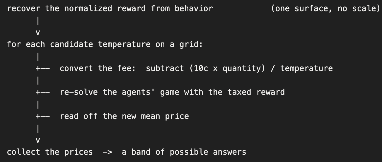
The procedure, start to finish, for the per-unit fee:
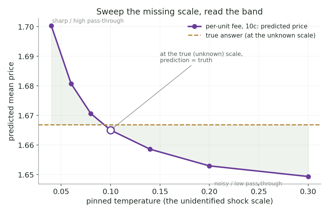
The downward-sloping curve is the impact of the per-unit fee: its predicted impact on price runs from about 1.70 at a low temperature, where sellers price sharply and pass the fee straight through, down to about 1.65 at a high temperature, where their algorithms are noisy and barely react. That five-cent spread is the honest width of the answer. The flat line is the profit commission from lever one, which needs no conversion and so returns a single value at every temperature. And the dashed line is the true price response, which the sweep brackets: at the true (but unknowable) scale, the prediction sits right on it.
The width of that band represents the honest level of uncertainty we face. A single value means the marketplace owner has a number and should trust it. A wide band means the owner has a range, and the honest report is the range, together with a statement of exactly how much one outside assumption about the dollar scale would buy by how far it collapses the interval. That is not a failure to answer. It is a precise map of which rule changes the data can price outright and which it can only bound.
The core question, answered honestly
The marketplace owner's question was: can I predict how participants respond when I change the rules? The answer is now specific rather than hopeful. For some changes, yes, exactly, with a number that does not depend on anything I cannot measure. For others, only within a band, and I can tell you the band and its endpoints. For a few, not without an assumption no amount of watching will ever justify. The agents will not know when the rules shift, because they are continuously learning and updating, so I do not have to model a moment of re-optimization. I just have to understand how these learners settle, and I can re-run the inference whenever I want and track them directly.
Humans still do not optimize. But we are handing the optimizing to things that do, tethered to what we want, and for those things the old assumptions are finally more than a convenient fiction. The apparatus I was trained on was not wrong about optimization. It was just early. It was waiting for optimizers to show up. What it still cannot do is turn behavior into a full set of primitives, because some of them are not in the behavior to be found. The advance is not that this limit disappears. It is that, for the first time, we can say precisely which questions it touches and which it does not, and sweep across the gap to bound the rest.
Some Technical Notes
The claim that reinforcement learning agent's choice rule and the econometrician's estimator are the same object, or rather that Maximum Causal Entropy IRL from machine learning and the dynamic discrete choice estimators from economics (the Nested Fixed Point algorithm, the Conditional Choice Probability method, and the Nested Pseudo-Likelihood algorithm) all belong to a single class of optimization problems, sharing a common objective, policy, and gradient, is due to:
Groeger, J., with N. Sanghvi, S. Usami, M. Sharma, and K. Kitani (2021). "Inverse Reinforcement Learning with Explicit Policy Estimates." Proceedings of the AAAI Conference on Artificial Intelligence, 35(11), 9472–9480. https://doi.org/10.1609/aaai.v35i11.17141
That paper is the bridge. Everything here, recovering the payoff from soft-Q pricing agents, reading the shock scale as the classical logit normalization, sorting counterfactuals by their invariance to it, is downstream of the fact that the two fields were solving the same inverse problem under different names. Once the estimators are known to coincide, the economics results about identification, normalization, and which counterfactuals survive an unidentified scale transfer directly onto the machine learning agents, which is the move the post is built on.
The supporting literature it connects sits on both sides of that bridge.
On the economics side, the dynamic discrete choice tradition: Rust (1987) on the nested fixed point and the logit-shock formulation; Hotz and Miller (1993) on inverting choice probabilities; Aguirregabiria and Mira (2002) on pseudo-likelihood; Magnac and Thesmar (2002) on what is and is not identified, and the necessity of normalizing the shock scale; Pesendorfer and Schmidt-Dengler (2008) on asymptotic least squares; and Kalouptsidi, Scott, and Souza-Rodrigues (2021) on which counterfactuals are identified when the payoff is not.
On the machine learning side, the entropy-regularized reinforcement learning tradition: Ziebart (2010) on maximum causal entropy IRL; Haarnoja et al. (2017) on soft Q-learning; and Geist, Scherrer, and Pietquin (2019) on regularized Markov decision processes.
On the learning-as-foundation side, the older idea that agents who estimate their environment can converge to equilibrium: Bray (1982) and Bray and Savin (1986) on least-squares learning of rational expectations, with the convergence machinery in Marcet and Sargent (1989); and, for the pricing environment specifically, Calvano, Calzolari, Denicolò, and Pastorello (2020) on Q-learning agents that learn to set supra-competitive prices.